Bipartite network projection and personal recommendation
本文最后更新于 2024年6月14日 晚上
Bipartite network projection and personal recommendation
论文要做什么?
这篇论文主要提出了一种加权方法(NBI),用来保留二分网络的原始信息(因为单模投影压缩二分网络会丢失信息) 。除此之外为了展示性能,用用户-电影数据比较了另外两种方法和本文提出方法的性能区别。
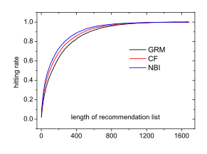
文章实验
数据集使用MovieLens
对比算法:
- GRM(Global Ranking Method)
- CF(Collaborative Filtering)
- NBI(Network-Based Inference)
实验结果:
NBI > CF > GRM
实验复现
导入的包
1
2
3
4
5
6
import networkx as nx
import matplotlib.pyplot as plt
import numpy as np
import pandas as pd
import pathlib
%matplotlib inline读取数据
1
2
3
4
5
6
7
8
users = pd.read_csv(DATA_DIR / 'u.user', sep='|', names=['user_id', 'age', 'gender', 'occupation', 'zip_code'])
occupation = pd.read_csv(DATA_DIR / 'u.occupation', header=None, names=['occupation'])
movies = pd.read_csv(DATA_DIR / 'u.item', sep='|',
names=['movie_id', 'movie_title', 'release_date', 'video_release_date', 'IMDb_URL', 'unknown', 'Action', 'Adventure', 'Animation', 'Children\'s', 'Comedy', 'Crime', 'Documentary', 'Drama', 'Fantasy', 'Film-Noir', 'Horror', 'Musical', 'Mystery', 'Romance', 'Sci-Fi', 'Thriller', 'War', 'Western'], encoding='ISO-8859-1') # 列明在数据集的README,编码utf8打不开,PyCharm给建议的ISO-8859-1
DataIndex = 1 # 数据集给了u1-u5,不知道为什么要分
train = pd.read_csv(DATA_DIR / f'u{DataIndex}.base', sep='\t', names=['user_id', 'item_id', 'rating', 'timestamp'])
test = pd.read_csv(DATA_DIR / f'u{DataIndex}.test', sep='\t', names=['user_id', 'item_id', 'rating', 'timestamp'])数据预处理
这里创建了一张
n*m大小的矩阵collected_frame,其中n为电影的总数,m为用户总数,表中数据为1表示用户“收集/收藏”了这部电影,0表示未收藏。即
collected_frame.loc[i,j]=1表示用户j+1收集了电影i+1(这里+1是因为电影和用户id从1开始,而数组从0开始)根据论文作者说法,电影评分\(rating \geq 3\)表示用户收藏了这部电影
1
2
3
4
5
collected_frame = pd.DataFrame(np.zeros((len(movies), len(users))))
for i in range(len(train)):
if train.rating[i] < 3:
continue
collected_frame.iloc[train.item_id[i] - 1, train.user_id[i] - 1] = 1L是推荐列表长度,用作实验结果的x轴
1
L = np.floor(np.linspace(0, len(movies) + 1, min(50, len(movies) + 1))).astype(int)GRM算法推荐
- GRM算法是将所有电影计算受欢迎程度,也就是有多少人收藏了这部电影,然后根据这个值从高到低进行推荐
- 创建一个长度为
n的数组,用于存放每个电影的受欢迎程度
1
2
#collected_frame.sum(axis='columns') # 将collected_frame按列求和(每一行的值加一块作为这一行的受欢迎程度)
grm_frame_sorted = collected_frame.loc[collected_frame.sum(axis='columns').sort_values(ascending=False).index, :] # 将预处理后得到的collected_frame根据受欢迎程度从高到低排序- 实现算法
1
2
3
4
5
6
7
8
9
def grm(user_id: int, L: int = 5) -> list[int]:
res = []
i = 0
while (len(res) < L and i < len(grm_frame_sorted)): # 保证L个推荐,i表示当前遍历到的电影
row = grm_frame_sorted.iloc[i]
if row.iloc[user_id - 1] != 1: # 如果用户没有看过该电影
res.append(grm_frame_sorted.index[i] + 1) # 添加到推荐列表中
i += 1
return resCF算法推荐
CF算法是找最相似的人收集的电影
使用一个\(m\times m\)的表
similar_martix存放用户间的相似度,其中similar_martix[i-1][j-1]表示用户i和用户j之间的相似度。用户间相似度计算
similar_martix[i-1][j-1]=\(s_{ij} = \frac{\sum_{l=1}^na_{li}a_{lj}}{min\{k(u_i), k(u_j)\}}\)1
2
3
4
5
6
7
8
9
10
11similar_martix = np.zeros((len(users), len(users)))
for i in range(len(users)):
for j in range(len(users)):
if j <= i: # 矩阵是对称的,算一半就行。i==j时设为0,因为下一步公式中要求l≠i
continue
d = min(collected_frame.loc[:, i].sum(), collected_frame.loc[:, j].sum()) # 这是公式的分母部分
if d == 0:
continue
# similar_martix[i, j] = sum([collected_frame.loc[l, i] * collected_frame.loc[l, j] for l in range(len(movies))]) / d
similar_martix[i,j] = collected_frame.loc[:,i].T.dot(collected_frame.loc[:,j]) / d # 使用矩阵运算代替上面注释掉的计算,可以提高运行速度
similar_martix[j, i] = similar_martix[i, j] # 矩阵是对称的公式中分子部分的\(\sum_{l=1}^na_{li}a_{lj}\)表示用户
i和用户j同时收集的电影的个数,只有两个都收集时才会使\(a_{li}a_{lj}=1\)计算对象预测得分
这里用函数
cf_value来计算对象的预测得分\(v_{ij}\)\(v_{ij} = \frac{\sum_{l=1,l \neq i}^m s_{li}a_{jl}}{\sum_{l=1,l\neq i}^ms_{li}}\)
1
2
3
4
5
6
7
8def cf_value(i,j):
# 由于上一步similar_martix中对角线部分值为0,所以可以直接点乘,不用担心l≠i的要求
n = np.dot(similar_martix[i-1], collected_frame.iloc[j-1])
d = np.sum(similar_martix[i-1])
if d == 0:
return 0
else:
return n / d实现算法
1
2
3
4
5
6
7
8
9
10
11
12
13
14def cf(user_id: int, L: int = 5) -> list[int]:
# 对象的分表,计算每个对象对于被推荐用户的得分
v_set = np.array([cf_value(user_id, j) for j in range(1, len(movies) + 1)])
# 用户已经收集的对象
collected = collected_frame.loc[:, user_id - 1].where(lambda x: x == 1).dropna().index.to_numpy()
# 将得分表中已经收集的对象的值设为-1
v_set[collected] = -1
# 排序后已经收集的对象一定在最后
v_set = np.argsort(-v_set)
# 将列表最后已收集的对象去除
v_set = v_set[:-1 * len(collected)]
# 转化为对象的id
v_set += 1
return v_set[:L]
NBI算法推荐
利用二分网络计算相似度进行推荐
假设被推荐用户的ID为
u先找到所有
u所收集的对象u_neighbors,并赋值1。这里代码实现使用f_o_initial记录u_neighbors获得的值将对象的值均分给收集此对象的用户
- 对于节点
i, 将节点的资源(上一步被赋的值)均分给连接的User节点,也就是\(被连接的节点资源 += \frac{i的资源}{i的度}\)
- 对于节点
将用户的资源再以同样的方式分给对象
将对象按所获得的资源量进行排序,去除用户已关联的对象后给出推荐列表
1
2
3
4
5
6
7
8
9
10
11
12
13
14
15
16
17
18
19
20
21
22
23
24
25
26
27
28
29
30
31
32
33
34
35
36
37
38
39
40def nbi(G, user_id: int, u_num: int = 983, o_num: int = 1682)->list:
"""
计算指定用户user_id的推荐列表
:param G: 用户-物品二分图
:param user_id: 用户ID
:param u_num: 总用户数
:param o_num: 总物品数
:return: 推荐物品列表
"""
f_o_initial = np.zeros(o_num) # 存放Object开始时的资源
f_u = np.zeros(u_num) # 存放Object转到Users时的资源
f_o = np.zeros(o_num) # 存放Users转到Objects时的资源,也是最终的推荐列表
# 初始化Object的资源,将被推荐用户所关联的资源全部赋值为1
u_neighbors = np.array(list(G.neighbors(user_id))) - u_num - 1
f_o_initial[u_neighbors] += 1
# 第一步:资源从Object集到User集O-->U
for o, fo in enumerate(f_o_initial): # 这里也可以循环range(u_num+1,u_num+o_num+1)
o_node_id = o + u_num + 1 # 对象节点id
o_degree = G.degree(o_node_id)
if o_degree == 0 or fo==0: # 度为零会导致后边报错,资源为0则没必要计算
continue
neighbors = np.array(list(G.neighbors(o_node_id))) - 1
f_u[neighbors] += fo / o_degree
# 第二步:资源从User集到Object集U-->O
for u, fu in enumerate(f_u):
u_node_id = u + 1
u_degree = G.degree(u_node_id)
if u_degree == 0 or fu==0:
continue
neighbors = np.array(list(G.neighbors(u_node_id))) - u_num - 1 # 因为Object的id排在user后面,所以要多减去u_num
f_o[neighbors] += fu / u_degree
f_o[u_neighbors] = -1 # 将值设置为-1,下一步排序时就一定会被放在末尾
f_o = np.argsort(-f_o)
f_o = f_o[:-1 * len(u_neighbors)] # 去掉末尾的几个(用户已收集的Object)
f_o += 1 # 将数组的角标转化为Object的id
return f_o计算各参数的代码如下:
1
2
3
4
5
6
7
8
9
10
11
12
13
14
15
16
17
18
19
20
21
22
23
24
25
26
27
28
29
30
31
32
33
34
35
36
37
38
39
40
41
42
43
44
45
46
47
48
49
50
51
52
53
54
55
56
57
58
59
60
61
62hitting_rate_cf = np.zeros(len(L))
hitting_rate_grm = np.zeros(len(L))
hitting_rate_nbi = np.zeros(len(L))
r_set_cf = np.zeros(len(test))
r_set_nbi = np.zeros(len(test))
r_set_grm = np.zeros(len(test))
user_num = 0
for i, (idx, u) in enumerate(tqdm(users.iterrows(), total=users.shape[0])):
# print(f'当前计算用户:{u.user_id}')
test_list = test.where((test.user_id == u.user_id) & (test.rating >= 3)).dropna()
true_list = set(test_list.item_id.tolist())
if len(test_list) == 0:
continue
forecast_grm = grm(u.user_id, L=max(L))
forecast_cf = cf(u.user_id, L=max(L))
forecast_nbi = nbi(G, u.user_id, u_num=len(users), o_num=len(movies))
for il in range(len(L)):
tmp_forecast_grm = forecast_grm[:L[il]]
tmp_forecast_cf = forecast_cf[:L[il]]
tmp_forecast_nbi = forecast_nbi[:L[il]]
hit_grm = len(set(tmp_forecast_grm).intersection(true_list)) / len(true_list)
hit_cf = len(set(tmp_forecast_cf).intersection(true_list)) / len(true_list)
hit_nbi = len(set(tmp_forecast_nbi).intersection(true_list)) / len(true_list)
hitting_rate_grm[il] += hit_grm
hitting_rate_cf[il] += hit_cf
hitting_rate_nbi[il] += hit_nbi
forecast_grm = list(forecast_grm)
forecast_cf = list(forecast_cf)
forecast_nbi = list(forecast_nbi)
for j, t in test_list.iterrows():
if t.rating < 3:
continue
try:
positions_grm = forecast_grm.index(t.item_id) + 1
except ValueError:
positions_grm = 0
try:
positions_cf = forecast_cf.index(t.item_id) + 1
except ValueError:
positions_cf = 0
try:
positions_nbi = forecast_nbi.index(t.item_id) + 1
except ValueError:
positions_nbi = 0
r_set_grm[j] = positions_grm / len(forecast_grm)
r_set_cf[j] = positions_cf / len(forecast_cf)
r_set_nbi[j] = positions_nbi / len(forecast_nbi)
user_num += 1
nonzero_count = test.where(test.rating >= 3).count()['user_id']
r_set_grm = np.sort(r_set_grm)
r_average_grm = np.sum(r_set_grm) / nonzero_count
r_set_cf = np.sort(r_set_cf)
r_average_cf = np.sum(r_set_cf) / nonzero_count
r_set_nbi = np.sort(r_set_nbi)
r_average_nbi = np.sum(r_set_nbi) / nonzero_count
hitting_rate_grm /= user_num
hitting_rate_cf /= user_num
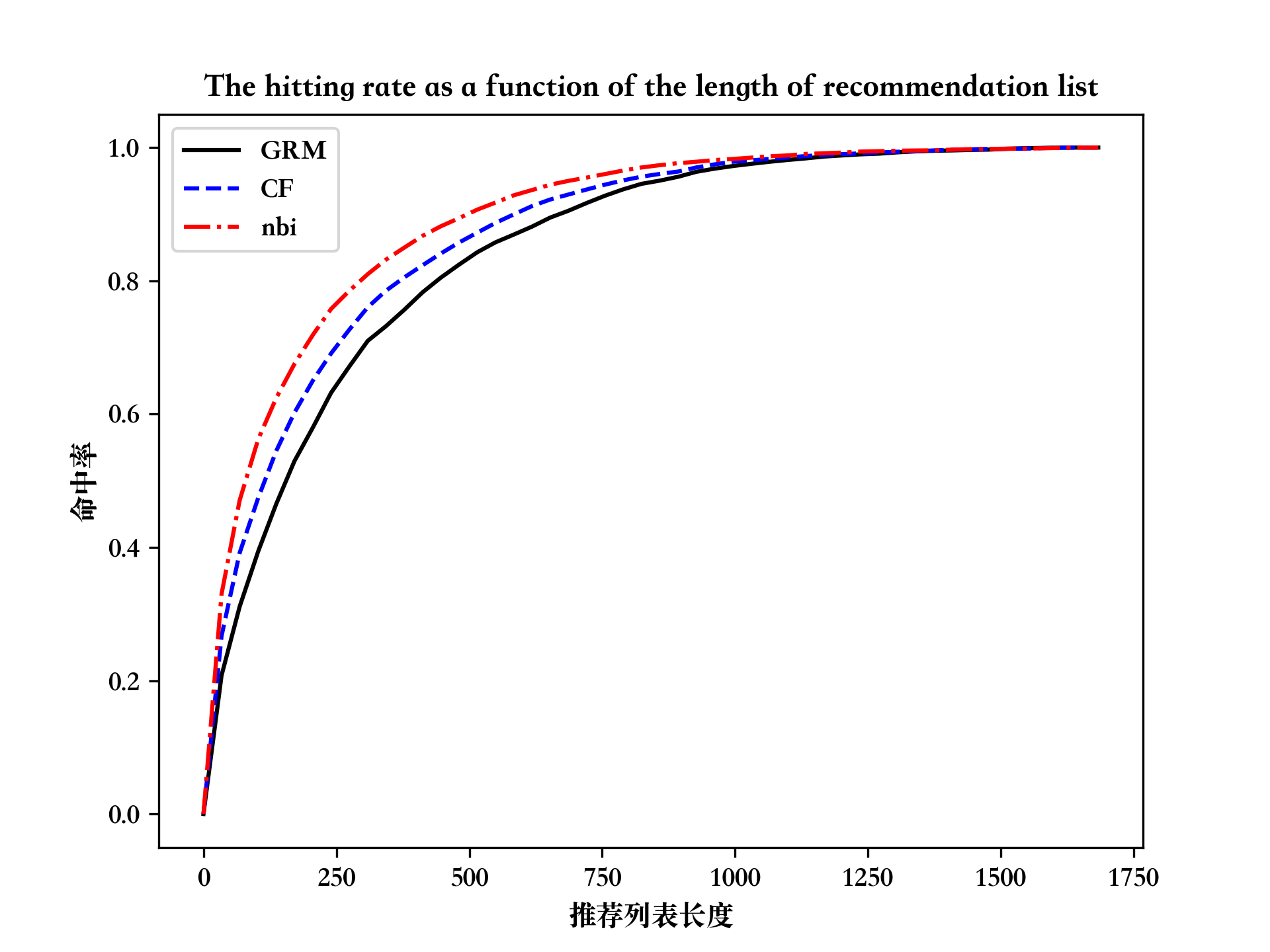
hitting_rate_nbi /= user_num三种算法的对比结果图
1
2
3
4
5
6
7
8
plt.plot(L, hitting_rate_grm, color='black', label='GRM')
plt.plot(L, hitting_rate_cf, color='blue', label='CF', linestyle='--')
plt.plot(L, hitting_rate_nbi, color='red', label='nbi', linestyle='-.')
plt.legend(['GRM', 'CF', 'nbi'])
plt.title('The hitting rate as a function of the length of recommendation list')
plt.xlabel('推荐列表长度')
plt.ylabel('命中率')
plt.savefig('recommend_functions.png',dpi=300)The predicted position of each entry in the probe ranked in the ascending order(按升序排列的探测器中每个条目的预测位置)
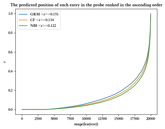
1
2
3
4
5
6
7
8plt.plot(range(len(test)), r_set_grm, label=f'GRM <r>={r_average_grm:.3f}')
plt.plot(range(len(test)), r_set_cf, label=f'CF <r>={r_average_cf:.3f}')
plt.plot(range(len(test)), r_set_nbi, label=f'NBI <r>={r_average_nbi:.3f}')
plt.legend([f'GRM <r>={r_average_grm:.3f}', f'CF <r>={r_average_cf:.3f}', f'NBI <r>={r_average_nbi:.3f}'])
plt.title('The predicted position of each entry in the probe ranked in the ascending order')
plt.xlabel('range(len(test))')
plt.ylabel('r')
plt.show()